 I can see that most midfielders and forwards group together, with some
defenders more similar to goalkeepers and others more similar to
midfielders.
I can see that most midfielders and forwards group together, with some
defenders more similar to goalkeepers and others more similar to
midfielders.UMAP (Uniform Manifold Approximation and Projection) is basically a way to translate high-dimensional data in a lower dimension representation by first creating a topological graph: each point has a local radius determined by it’s nth nearest neighbour, and is made ‘fuzzy’, where radii have a lower likelihood of connection as they get larger.
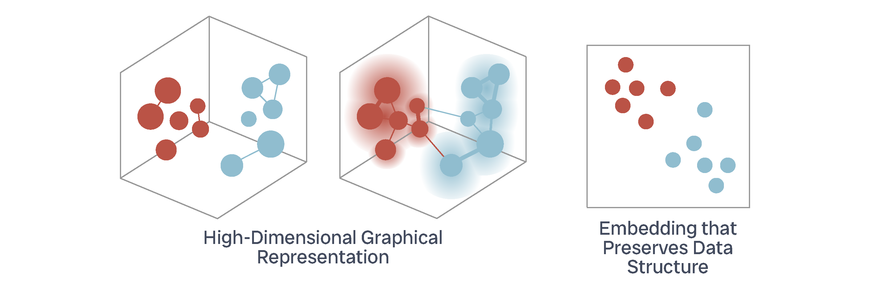
This is like a weighted graph, with edges representing a likelihood of connection. With this high-dimensional weighted graph, UMAP then creates a lower-dimension version, which it optimises to be as structurally similar to the high-dimensional graph as possible. Because UMAP forces each point to be connected to at least one neighbour (it’s nearest), it represents local structures as well as global structure. However, this means that ‘distance’ between points in a UMAP plot doesn’t really mean anything.
I really like using UMAP paired with a clustering method like DBSCAN to investigate patterns in high-dimensional data. Here I want to look at whether there are ‘clusters’ of player profiles in the Premier League. The utility of this is seeing which players are similar to each other.
First I am going to read in some Premier League data from this season!
# Packages
library(tidyverse)
library(extrafont)
library(ggrepel)
library(dplyr)
library(umap)
library(dbscan)

# Read data
Path <- '/Users/alicesmail/Desktop/Programming/GitHubPage/FPL/2024-2025-Data/'
PlayerData <- read_csv(paste0(Path, "FPL-Gameweeks-29.csv"))
head(as.data.frame(PlayerData[6:11]))
## second_name team team_code team_name team_short_name web_name
## 1 Ferreira Vieira 1 3 Arsenal ARS Fábio Vieira
## 2 Fernando de Jesus 1 3 Arsenal ARS G.Jesus
## 3 dos Santos Magalhães 1 3 Arsenal ARS Gabriel
## 4 Havertz 1 3 Arsenal ARS Havertz
## 5 Hein 1 3 Arsenal ARS Hein
## 6 Timber 1 3 Arsenal ARS J.TimberHere I am just using dplyr functions to summarise different metrics for each player across the season so far:
# Summarise data
PlayerDataSum <- PlayerData %>%
  group_by(web_name, team_short_name, position) %>%
  summarise(goals_scored=sum(goals_scored), assists=sum(assists),
            creativity=sum(creativity), xA=sum(expected_assists),
            xG=sum(expected_goals), influence=sum(influence),
            threat=sum(threat), minutes=sum(minutes)) %>%
  unique() %>% filter(minutes>90*10)

# Get statistics per 90 minutes
PlayerDataSum <- PlayerDataSum %>%
  group_by(web_name, team_short_name, position) %>%
  summarise(creat90=round((creativity/minutes)*90,2),
            influ90=round((influence/minutes)*90,2),
            thr90=round((threat/minutes)*90,2),
            ast90=round((assists/minutes)*90,2),
            gls90=round((goals_scored/minutes)*90,2),
            xA90=round((xA/minutes)*90,2),
            xG90=round((xG/minutes)*90,2)) %>%
  rename('name'='web_name',
         'team'='team_short_name')
Now I have got a few different per 90 metrics for each player:
# View
PlayerDataSum %>% arrange(-xG90) %>% as.data.frame() %>% head()
## name team position creat90 influ90 thr90 ast90 gls90 xA90 xG90
## 1 Haaland MCI FWD 11.74 32.89 51.10 0.11 0.76 0.06 0.75
## 2 M.Salah LIV MID 32.33 50.31 58.45 0.60 0.95 0.24 0.75
## 3 Isak NEW FWD 20.67 38.25 42.79 0.22 0.83 0.14 0.68
## 4 Watkins AVL FWD 12.66 27.02 42.02 0.26 0.57 0.07 0.60
## 5 Wissa BRE FWD 12.04 25.57 35.56 0.13 0.55 0.06 0.58
## 6 N.Jackson CHE FWD 16.53 26.03 44.30 0.31 0.47 0.09 0.56Next I just want to make sure each row has a unique rowname as some players have the same web name.
# Unique rownames
PlayerDataSum <- PlayerDataSum %>% as.data.frame()
row.names(PlayerDataSum) <- paste(make.unique(PlayerDataSum$name))With this input data I can select the columns I want to input into the UMAP and perform the UMAP!
# Perform UMAP
set.seed(1)
PlayerDataUMAP <- PlayerDataSum %>%
  select(-c(name, position, team)) %>%
  select(where(is.numeric)) %>%
  scale() %>%
  umap(preserve.seed=T)

# Add info
PlayerDataUMAPPlot <- PlayerDataUMAP$layout %>% as.data.frame() %>%
  rename(UMAP1='V1', UMAP2='V2') %>% as.data.frame()
PlayerDataUMAPPlotAll <- merge(PlayerDataUMAPPlot %>% rownames_to_column('ID'),
                               PlayerDataSum %>% rownames_to_column('ID'))
To visualise the results I can just plot the UMAP coordinates on a scatter plot.
# Palette
palette <- list(colorRampPalette(colors=c('#ba5346', '#cfc963', '#75a450', '#90bdcf'))(4))

# Plot
ggplot(PlayerDataUMAPPlotAll, aes(x=UMAP1, y=UMAP2, colour=position))+
  geom_point(size=4, alpha=0.75)+
  theme_classic()+
  theme(text=element_text(family='Roboto',size=14))+
  scale_colour_manual(values=palette[[1]])+
  labs(colour='Position')
I can see that most midfielders and forwards group together, with some
defenders more similar to goalkeepers and others more similar to
midfielders.
Next I can apply DBSCAN clustering to the UMAP coordinates identify similar players.
# DBSCAN
DB <- dbscan(PlayerDataUMAPPlotAll %>% select(UMAP1, UMAP2), eps=0.4, minPts=5)
PlayerDataUMAPPlotAll$Cluster <- DB$cluster

# Palette
palette <- list(colorRampPalette(colors=c('#ba5346', '#cfc963', '#75a450', '#90bdcf'))(max(PlayerDataUMAPPlotAll$Cluster)+1))

# Plot
ggplot(PlayerDataUMAPPlotAll, aes(x=UMAP1, y=UMAP2, colour=as.factor(Cluster)))+
  geom_point(size=4, alpha=0.75)+
  theme_classic()+
  theme(text=element_text(family='Roboto',size=14))+
  scale_colour_manual(values=c('#ebebeb', palette[[1]]))+
  labs(colour='Group')+
  guides(colour='none')
I can now inspect some of the groups! Here, group 6 is made up of central/defensive midfielders like Anderson, Kovačić and Rice, as well as more attacking defenders, like Hall, Robinson, Pedro Porro and Trent Alexander-Arnold.
# Group 6
PlayerDataUMAPPlotAll %>% filter(Cluster==6) %>%
  select(name, position, team, creat90, influ90, thr90, ast90, gls90, xA90, xG90) %>%
  arrange(-influ90) %>% head(n=10)
## name position team creat90 influ90 thr90 ast90 gls90 xA90 xG90
## 1 Alexander-Arnold DEF LIV 33.27 27.75 9.74 0.25 0.08 0.27 0.06
## 2 Robinson DEF FUL 21.57 26.87 6.31 0.35 0.00 0.12 0.02
## 3 Pedro Porro DEF TOT 29.42 26.60 7.39 0.20 0.08 0.14 0.06
## 4 Kovačić MID MCI 24.16 23.42 8.05 0.11 0.21 0.14 0.08
## 5 Hall DEF NEW 23.08 23.10 5.27 0.29 0.00 0.15 0.02
## 6 Tielemans MID AVL 29.41 22.75 7.95 0.14 0.07 0.18 0.09
## 7 Anderson MID NFO 23.30 22.20 10.06 0.27 0.05 0.14 0.06
## 8 Christie MID BOU 23.51 21.88 12.69 0.13 0.09 0.12 0.09
## 9 Rice MID ARS 31.82 21.79 10.86 0.21 0.08 0.21 0.08
## 10 Bellegarde MID WOL 23.35 20.94 12.18 0.42 0.14 0.17 0.08Meanwhile group 2 is made up of creative midfielders, especially wingers like Elanga, Jacob Murphy, Amad and Saka, who have high xA and assists.
# Group 2
PlayerDataUMAPPlotAll %>% filter(Cluster==2) %>%
  select(name, position, team, creat90, influ90, thr90, ast90, gls90, xA90, xG90) %>%
  arrange(-ast90) %>% head(n=8)
## name position team creat90 influ90 thr90 ast90 gls90 xA90 xG90
## 1 Saka MID ARS 44.72 36.64 42.87 0.78 0.35 0.40 0.30
## 2 Savinho MID MCI 33.37 20.92 34.42 0.58 0.06 0.31 0.27
## 3 Son MID TOT 34.42 29.93 30.71 0.49 0.34 0.23 0.32
## 4 Gibbs-White MID NFO 27.18 23.62 22.11 0.45 0.22 0.18 0.18
## 5 J.Murphy MID NEW 21.44 24.64 19.44 0.43 0.27 0.20 0.21
## 6 B.Fernandes MID MUN 38.69 32.48 18.34 0.42 0.30 0.21 0.32
## 7 Amad MID MUN 31.24 29.23 26.98 0.40 0.34 0.19 0.23
## 8 Elanga MID NFO 28.65 23.57 19.80 0.39 0.24 0.18 0.19I can also use this information to identify players with similar playing profiles. Looking at defenders, Kerkez has similar statistics to Aït-Nouri, Wan-Bissaka, Ashley Young and Muñoz - these players have quite high creativity for defenders, with relatively high goals and assists per 90 compared to their xG and xA.
# Which defenders have similar statistics to Kerkez?
PlayerDataUMAPPlotAll %>%
  filter(Cluster==PlayerDataUMAPPlotAll[grep("Kerkez", PlayerDataUMAPPlotAll$name),]$Cluster & position=='DEF') %>%
  select(name, position, team, creat90, influ90, thr90, ast90, gls90, xA90, xG90)
## name position team creat90 influ90 thr90 ast90 gls90 xA90 xG90
## 1 Aït-Nouri DEF WOL 14.83 21.69 10.65 0.19 0.11 0.07 0.07
## 2 Kerkez DEF BOU 15.88 20.14 6.95 0.21 0.07 0.07 0.02
## 3 Muñoz DEF CRY 17.52 22.96 15.24 0.19 0.12 0.09 0.16
## 4 Wan-Bissaka DEF WHU 14.60 21.87 5.18 0.11 0.07 0.08 0.04
## 5 Young DEF EVE 16.20 21.09 2.67 0.23 0.06 0.11 0.02Finally, Chris Wood is most similar to several other attackers, including Haaland, Mateta and Wissa. These players all have very high xG and threat, but relatively low xA and creativity (with the exception of Salah!).
# Which strikers have similar statistics to Chris Wood?
PlayerDataUMAPPlotAll %>%
  filter(Cluster==PlayerDataUMAPPlotAll[grep("Wood", PlayerDataUMAPPlotAll$name),]$Cluster) %>%
  select(name, position, team, creat90, influ90, thr90, ast90, gls90, xA90, xG90) %>%
  arrange(-gls90) %>% head(n=8)
## name position team creat90 influ90 thr90 ast90 gls90 xA90 xG90
## 1 M.Salah MID LIV 32.33 50.31 58.45 0.60 0.95 0.24 0.75
## 2 Isak FWD NEW 20.67 38.25 42.79 0.22 0.83 0.14 0.68
## 3 Haaland FWD MCI 11.74 32.89 51.10 0.11 0.76 0.06 0.75
## 4 Wood FWD NFO 8.66 28.58 29.27 0.12 0.69 0.04 0.42
## 5 Beto FWD EVE 8.61 27.18 43.73 0.00 0.59 0.02 0.52
## 6 Watkins FWD AVL 12.66 27.02 42.02 0.26 0.57 0.07 0.60
## 7 Wissa FWD BRE 12.04 25.57 35.56 0.13 0.55 0.06 0.58
## 8 Mateta FWD CRY 15.09 24.04 26.55 0.08 0.51 0.09 0.48Here I have applied UMAP and DBSCAN to identify collections of Premier League players with similar statistics.